
I was always good at math growing up, but it was never a main interest of mine. Early into my college career, it somehow found its way as my passion, and I decided to abandon my pre-med biology major to study mathematics full time. It wasn’t long before I began taking notice of how people either loved math, or they absolutely hated it, and would say something along the lines of “I’m just not a math person”.
I’ve always assumed that these people just never gave themselves the oppurtunity to truly enjoy mathematics because they never legitimately tried to conceptualize the material and do well. But then I got thinking, is “I’m just not a math person” a legitimate explanation for failing grades? Is mathematical ability genetic? Is it situational?
In this project, I attempt to build a machine learning model that uses seemingly irrelevant information about a student to predict their mathematical ability.
Data Exploration
The dataset I will be using is one from the UCI repository that contains the final scores of 395 students at the end of a math program, and several features that may or may not impact the futures of these young adults. The data consists of 30 predictive features, columns for the two term grades, and the final grade (G1, G2, and G3, respectively).

The 30 features detail the social lives, home lives, family dynamics, and the future aspirations of the students. For obvious reasons, the two term grades, G1 and G2, will not be included in the actual model.
Overview :
1. Variable Identification
2. Univariate Analysis
3. Bivariate Analysis
a. Target Correlation
b. Feature Correlation
1
2
3
4
5
6
7
import numpy as np
import pandas as pd
import matplotlib.pyplot as plt
import seaborn as sns

# load in dataset
stud = pd.read_csv('student-math.csv')
Feature Identification
The 30 predictive features are all categorical, and they contain a mix of numeric and nonnumeric entries.
Ordinal Features:
- age - student’s age (numeric: from 15 to 22)
- Medu - mother’s education (numeric: 0– none, 1- primary education (4th grade), 2- 5th to 9th grade, 3- secondary education, or 4- higher education)
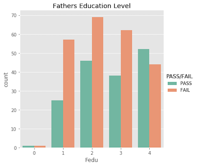
- Fedu - father’s education (numeric: 0– none, 1- primary education (4th grade), 2- 5th to 9th grade, 3- secondary education, or 4- higher education)
- traveltime - home to school travel time (numeric: 1 - 1 hour)
- studytime - weekly study time (numeric: 1 - 10 hours)
- failures - number of past class failures (numeric: n if 1<=n<3, else 4)
- famrel - quality of family relationships (numeric: from 1 - very bad to 5 - excellent)
- freetime - free time after school (numeric: from 1 - very low to 5 - very high)
- goout - going out with friends (numeric: from 1 - very low to 5 - very high)
- Dalc - workday alcohol consumption (numeric: from 1 - very low to 5 - very high)
- Walc - weekend alcohol consumption (numeric: from 1 - very low to 5 - very high)
- health - current health status (numeric: from 1 - very bad to 5 - very good)
- absences - number of school absences (numeric: from 0 to 93)
Nominal Features:
- school - student’s school (binary: ‘GP’ - Gabriel Pereira or ‘MS’ - Mousinho da Silveira)
- higher - wants to take higher education (binary: yes or no)
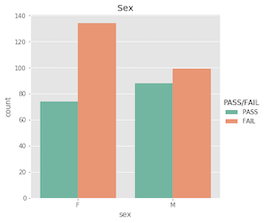
- sex - student’s sex (binary: ‘F’ - female or ‘M’ - male)
- address - student’s home address type (binary: ‘U’ - urban or ‘R’ - rural)
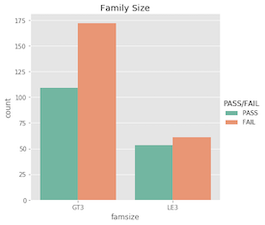
- famsize - family size (binary: ‘LE3’ - less or equal to 3 or ‘GT3’ - greater than 3)
- Pstatus - parent’s cohabitation status (binary: ‘T’ - living together or ‘A’ - apart)
- schoolsup - extra educational support (binary: yes or no)
- famsup - family educational support (binary: yes or no)
- paid - extra paid classes within the course subject (binary: yes or no)
- activities - extra-curricular activities (binary: yes or no)
- nursery - attended nursery school (binary: yes or no)
- internet - Internet access at home (binary: yes or no)
- romantic - with a romantic relationship (binary: yes or no)
- Mjob - mother’s job (nominal: ‘teacher’, ‘health’, civil ‘services’, ‘athome’, or ‘other’)
- Fjob - father’s job (nominal: ‘teacher’, ‘health’, civil ‘services’, ‘athome’, or ‘other’)
- reason - reason to choose this school (nominal: close to ‘home’, school ‘reputation’, ‘course’ preference or ‘other’)
- guardian - student’s guardian (nominal: ‘mother’, ‘father’ or ‘other’)
Grade Columns:
- G1 - first term grade (numeric: from 0 to 20)
- G2 - second term grade (numeric: from 0 to 20)
- G3 - final grade (numeric: from 0 to 20, output target)
At the top of the page is a link that will redirect you to the Kaggle post where this dataset can be found!
Univariate Analysis
The ordinal features contain only integer values, the nominal features contain only strings, and the grades are integer values in [0,20]. Let’s see how the three grade columns and the ordinal features are distributed.
1
2
plt.style.use('ggplot')
stud.hist(figsize= (20,15), color= 'b');
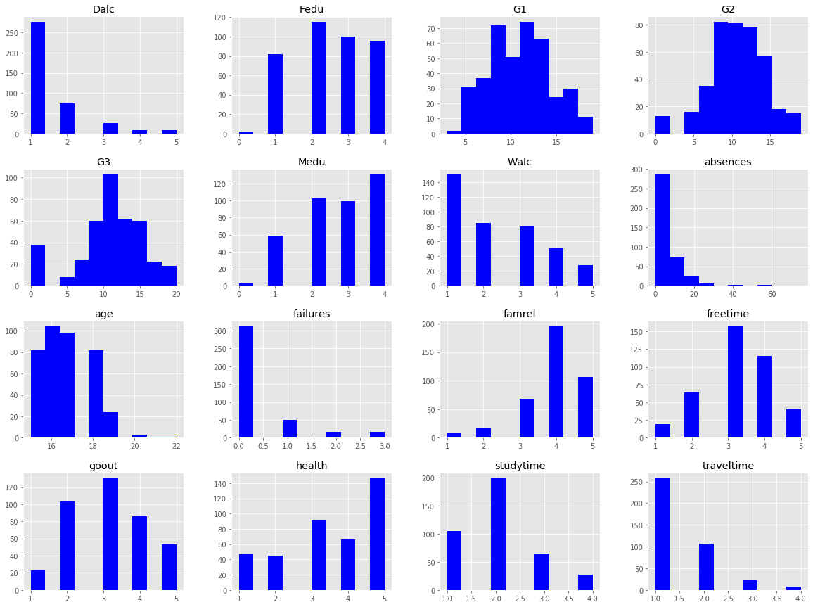
We can see right away that some of the features have categories with hardly any occurances (ex: Fedu, Medu, age, and absences), which isn’t surprising with a small sample size. These outliers may cause issues later on down the road, so I will take note of them now, and further evaluate them in the upcoming sections.
The shift in distributions of the three grades is rather interesting.
G1 - Low average, and high variance –> Students weren’t trying
G2 - Higher average, lower variance, and fewer failing grades –> Student’s began trying
G3 - Normally distributed (excluding the 0 values) with mean ~11
Bivariate Analysis
To determine whether a student either passed or failed the course, I need to define a threshold for G3. The minimum passing grade in the U.S. is typically considered to be a D-, so in our case, a 12/20 is the threshold for a minimum passing grade. (In this section the target labels are pass or fail, but in following sections they will just be 0’s and 1’s.)
1
stud['PASS/FAIL'] = stud['G3'].apply(lambda x: 'FAIL' if x<12 else 'PASS')
40% of the students classified as passing.
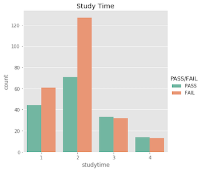
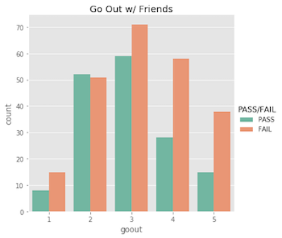
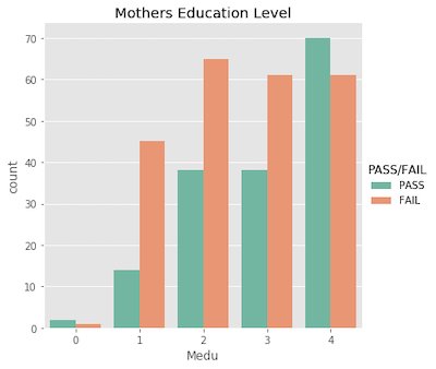
Target Correlation
First, I want to evaluate how the individual features correlate with the target variable. I will use seaborn to visualize the pass/fail frequencies of each feature.
You may have noticed that I only included the ordinal features in the previous section. To clarify, I did this because all but four of the nominal features are boolean, and can easily be described here.
Note that I did explore the entire set of features. Many of the features have low correlation with the target variable, and were uninteresting. So, for your viewing pleasure, I opted to exclude them – the interesting ones are plotted below!
Ordinal features…
Nominal features…
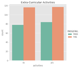
What’s important to acknowldge here is that a student’s pass/fail status is the outcome of an entire semester; it’s more complex than just a single test grade. Similarly, making a pass/fail prediction for a student is more difficult than just evaluating one feature!
With this being said, I suspect the features will show more correlation with the actual 0-20 final grade. Being in a relationship with someone probably won’t cause them to fail all of their classes, but it may very easily affect their final grade by a few points.
Feature Correlation
Now we’ll take a look at all corrolations. I’ll first need to encode the features having nonnumeric entries.
1
2
3
4
5
6
7
8
9
10
11
12
13
14
15
16
17
18
19
20
21
22
23
24
25
26
27
# drop term grades and old pass/fail target
stud = stud.drop(columns= ['G1', 'G2', 'PASS/FAIL'])

# define new target column
stud['target'] = stud['G3'].apply(lambda x: 0 if x<12 else 1)

# encode boolean categorical's with binary values
# school--> [0=GP, 1=MS]
stud['school'] = stud['school'].apply(lambda x: 0 if x=='GP' else 1)
# sex--> [0=F, 1=M]
stud['sex'] = stud['sex'].apply(lambda x: 0 if x=='F' else 1)
# address--> [0=U, 1=R]
stud['address'] = stud['address'].apply(lambda x: 0 if x=='U' else 1)
# famsize--> [0=LE3, 1=GT3]
stud['famsize'] = stud['famsize'].apply(lambda x: 0 if x=='LE3' else 1)
# Pstatus--> [0=T, 1=A]
stud['Pstatus'] = stud['Pstatus'].apply(lambda x: 0 if x=='T' else 1)

# yes/no boolean features--> [0=no, 1=yes]
yesno_feats = ['schoolsup','famsup','paid','activities','nursery','internet','romantic','higher']
for feat in yesno_feats:
    stud[feat] = stud[feat].apply(lambda x: 0 if x=='no' else 1)

# encoding multi-categorical features (alphabetically) to integer values
nominal_cols = ['Mjob','Fjob','reason', 'guardian']
for col in nominal_cols:
    stud[col] = stud[col].astype('category').cat.codes
To emphasize on my prior statement, notice how the correlations with the final grade seem more logical than with the 0-1 target variable.
1
2
3
4
5
# feature correlation to target variable
print(stud.corr()['target'].sort_values(ascending= False))

# feature correlation to target variable
print(stud.corr()['G3'].sort_values(ascending= False))
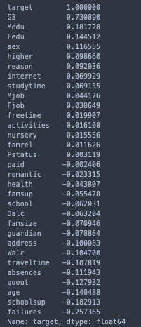
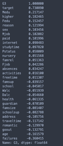
Hence, I’ll exclude the target variable and use G3 for the correlation matrix heatmap.
1
2
3
4
5
6
7
8
9
10
11
12
# sorted correlation matrix
G3_corr = stud.drop(columns= 'target').corr().sort_values(by= 'G3', ascending= False)
G3_corr = G3_corr[G3_corr.index.values]

# heatmap
plt.figure(figsize = (13,10))
sns.heatmap(G3_corr,
        vmax= .3,
        vmin= -.3,
        center= 0,
        xticklabels= 1,
        yticklabels= 1).set_title("Correlation Matrix");
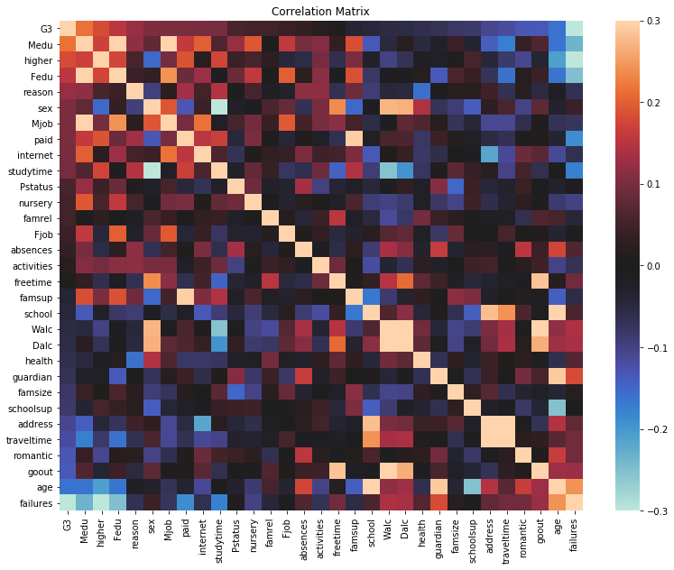
Positive Correlations:
-‘address’ and ‘traveltime’
-‘Dalc’, ‘Walc’, ‘goout’, and ‘freetime’
-‘famsup’ and ‘paid’
Negative Correlations:
-‘Dalc’, ‘Walc’, and ‘studytime’
-‘studytime’ and ‘sex’
These correlations seem reasonable, but the inverse correlation between the sex of a student and their average time spent studying is interesting. I’ll openly admit I’m not too surprised that we fall short to our female counterparts in this area, but what’s intersting is that..
1
2
3
4
5
6
7
print("On average, females spend",
      np.round((stud[stud['sex'] == 0]['studytime'].mean()/stud[stud['sex'] == 1]['studytime'].mean()-1)*100, 2),
      "% longer each week studying than males do. \nHowever,",
      np.round((stud[stud['sex'] == 1]['target'].sum()/stud[stud['sex'] == 1]['sex'].count())*100, 2),
     "% of males scored a passing grade, while the female percentage was only",
     np.round((stud[stud['sex'] == 0]['target'].sum()/stud[stud['sex'] == 0]['sex'].count())*100, 2),
     "%.")

Data Cleaning
With only 395 samples, I’d like to retain as many of them as possible. However, including underrepresented categories would ultimately result in a weak model.

Let’s take another look at the outliers we saw earlier.
1
2
3
# mother and father education level counts
print(stud['Medu'].value_counts())
print(stud['Fedu'].value_counts())
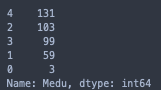
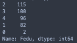
I will have to exclude the samples with 0 values for Medu/Fedu since they are greatly underrepresented, even in comparison to the next smallest categories.
1
2
3
# student age counts
print(stud['age'].value_counts())
sns.catplot(x = 'age', data= stud, hue= 'target', kind= 'count', hue_order= [1, 0], palette= 'Set2').set(title = 'Age')
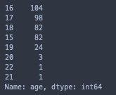
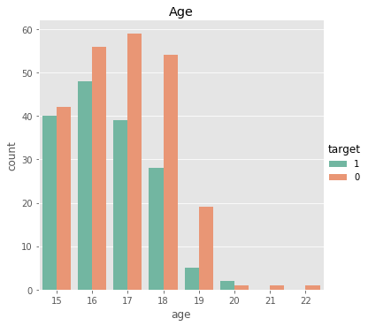
This feature is an interesting one, but it would be far-fetched to consider samples of sizes 3, 1, and 1 as accurate representations of any populations.
1
2
3
print(stud['absences'].value_counts())
sns.catplot(x = 'absences', data= stud, hue= 'target', kind= 'count', hue_order= [1, 0], palette= 'Set2', height= 7, aspect= 2).set(title = 'Absences')
plt.figure(figsize= (40,40))
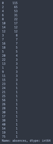
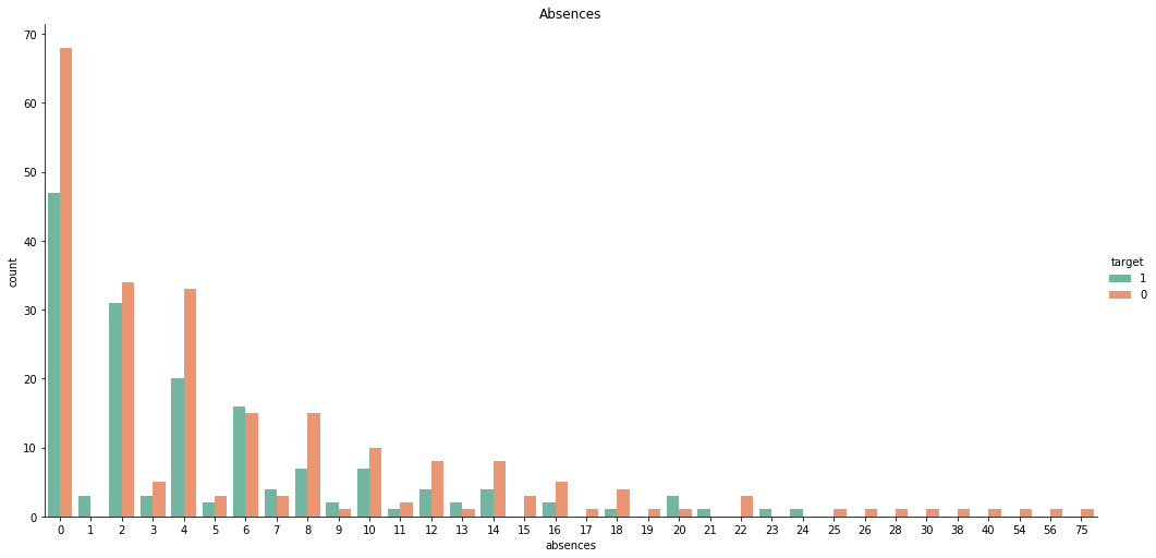
For ‘absences’, there are 46 samples in categories with no more than 5 total observations, and it’s less than ideal to drop them all. However, we can see that every instance where ‘absences’ > 24 resulted in the same outcome, a failed course. Hence, we can bin these values together. Although this only accounts for a portion of the underrepresented categories, it will still greatly improve the quality of the feature as a whole.
Although it seems natural to use ‘25’ to denote the 25+ bin, using a slighly larger integer, say 30, may benefit certain models where Euclidean distance is of importance.
1
2
3
4
5
6
7
8
9
10
11
12
13
14
15
16
17
# drop outlying samples
stud = stud[stud['Medu'] != 0]
stud = stud[stud['Fedu'] != 0]
stud = stud[stud['age'] != 20]
stud = stud[stud['age'] != 21]
stud = stud[stud['age'] != 22]

# make outlying 'absences' bin
stud['absences'] = stud['absences'].replace({25:30,
                                            26:30,
                                            28:30,
                                            30:30,
                                            38:30,
                                            40:30,
                                            54:30,
                                            56:30,
                                            75:30})
‘School’, ‘Pstatus’, and ‘higher’ also caught my attention earlier. See their bivariate graphs below.
1
2
3
sns.catplot(x = 'school', data= stud, hue= 'target', kind= 'count', hue_order= [1, 0], palette= 'Set2').set(title = 'School')
sns.catplot(x = 'Pstatus', data= stud, hue= 'target', kind= 'count', hue_order= [1, 0], palette= 'Set2').set(title = 'Parents: Together/Apart')
sns.catplot(x = 'higher', data= stud, hue= 'target', kind= 'count', hue_order= [1, 0], palette= 'Set2').set(title = 'Higher Education');
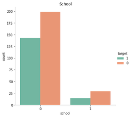
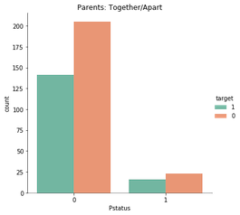
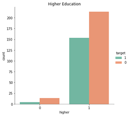
Each of these features have a dominate category with roughly 90% selection, so there’s not much, if any, information to be gained by their inclusion.
That is, consider the case where a student does not plan on furthering their education. They’ll mark ‘no’ for the feature ‘higher’, and many ML models would predecit they would fail solely due to the insufficient amount of data (18 of 395 students).
In sum, these features will be excluded from the analysis.
1
stud = stud.drop(columns=['school', 'Pstatus', 'higher'])
The resulting dataset has 27 features and 385 samples.
There are still a few features I feel aren’t relevant to passing a math class, but at this point, I cannot confirm that any one of the remaining features won’t be useful to the model.
Model Selection
- K-Nearest Neighbors
- Suport Vector Classifier
- Logistic Regression
- Decision Tree Classifier
- Gaussian Naive Bayes
- Random Forest Classifier
- Gradient Boosting Classifier
I will revisit feature selection soon, but for now I’ll evaluate the base performances of the seven classifiers listed above, and move forward with the top two.

If you’ve made it this far, you deserve a little honesty..
Prior to this very moment, my only exposure to machine learning was in mathematical statistics my junior year when we covered linear regression over the span of two 50-minute class periods. So, I’m sure there has to be better ways to go about selecting the best model for my problem, but I’m eager to learn, and I’m taking this project entirely as an opputtunity to learn!
Plus, this method will give me two seperate models to learn head-to-toe that I know will perform at least somewhat decent!
1
2
3
4
5
6
7
8
9
10
11
12
13
14
15
16
17
from sklearn.neighbors import KNeighborsClassifier
from sklearn.svm import SVC
from sklearn.linear_model import LogisticRegression
from sklearn.tree import DecisionTreeClassifier
from sklearn.naive_bayes import GaussianNB
from sklearn.ensemble import RandomForestClassifier
from sklearn.ensemble import GradientBoostingClassifier

# instantiate classifiers in a list
models = []
models.append(('KNN', KNeighborsClassifier()))
models.append(('SVC', SVC()))
models.append(('LR', LogisticRegression()))
models.append(('DT', DecisionTreeClassifier()))
models.append(('GNB', GaussianNB()))
models.append(('RF', RandomForestClassifier()))
models.append(('GB', GradientBoostingClassifier()))
The dataset is from Kaggle, but I’m not looking for a model that optimizes for accuracy at the expense of generality. I’m genuinely interested in the predictive capabilities of the 27 features, and would like for my model to be able to predict on new data as well.
For this to happen, I must estabalish a few precautionary measures.
High Variance - The dataset contains a less than preferrable number of samples, and because of this, testing accuracy will be highly subject to variation. I want the two best performing models of the group, but I do not want them if they can’t fit to new data. In attempt to mitigate this, I will use 10 repititions of 5-fold stratified cross validation when estimating each model’s out-of-sample accuracy.
Data Leakage - Instead of passing the stand alone models to cross_val_score, I will cross validate pipelines containing both the model, and the preprocessing steps. Thus, when the dataset is split into new training and test sets at each fold, the two sets will be preprocessed separately, and the chances of data leakage will be near-to-none!
1
2
3
4
5
6
7
8
9
10
11
12
13
14
15
16
17
18
19
20
21
22
23
24
25
26
27
28
29
30
31
32
33
34
35
36
37
38
39
40
41
42
43
from sklearn.pipeline import make_pipeline
from sklearn.preprocessing import  MinMaxScaler, OneHotEncoder
from sklearn.compose import make_column_transformer
from sklearn.model_selection import cross_val_score
from sklearn.model_selection import RepeatedStratifiedKFold
from sklearn.metrics import accuracy_score

# seperate target variable from feature set
Y = stud['target']
X = stud.drop(columns=['G3', 'target'])

# list of column labels with string values
# list of column labels with int values
cat_feats = X.select_dtypes('object').columns.to_list()
num_feats = X.select_dtypes('int').columns.to_list()

# 2-stage preprocessor
preprocessor = make_column_transformer(
    (MinMaxScaler(), num_feats),
    (OneHotEncoder(drop= 'first'), cat_feats))

# compute and store each model's average CV accuracy
names = []
scores = []
for name, model in models:
    pipe = make_pipeline(preprocessor, model)
    rep_kfold = RepeatedStratifiedKFold(n_splits= 5, n_repeats= 10, random_state= 777)
    score = cross_val_score(pipe, X, Y, cv=rep_kfold, scoring='accuracy').mean()

    names.append(name)
    scores.append(score)

# plot results
model_CVscores = pd.DataFrame({'Name': names, 'Score': scores})
model_CVscores.sort_values(by= 'Score', ascending= False).plot(kind='bar',
                                                               x= 'Name',
                                                               y= 'Score',
                                                               style= 'ggplot',
                                                               rot= 0,
                                                               legend= False)

# print results
print(model_CVscores.sort_values(by= 'Score', ascending= False))
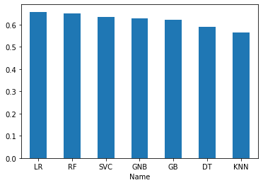
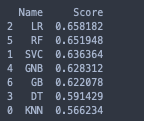
Logistic Regession and Random Forest seem to be the best two classifiers for the dataset. Both scored over 65% accuracy right out of the box with default parameters and no feature selection.

Constructing The Models
I’ll build the models on 70% of the data, and compare their predictions on the test set at the end. Here’s what this will look like:
1. Random Forest
a. Feature Selection
b. Hyperparameter Tuning
2. Logistic Regression
a. Feature Selection
b. Hyperparameter Tuning
3. Test the Models
First, I need to split the data into training and test sets.
1
2
3
4
5
6
7
8
from sklearn.model_selection import train_test_split

# instantiate base models
rfc = RandomForestClassifier()
logreg = LogisticRegression()

# 269-116 stratified sample split
X_train, X_test, Y_train, Y_test = train_test_split(X, Y, test_size= 0.3, stratify= Y, random_state= 777)
And just to verify that the target labels are split proportionally..
1
2
3
# proportions of passing students
print("Train Set: ", Y_train.sum()/Y_train.size)
print("Test Set: ", Y_test.sum()/Y_test.size)
1
2
Train Set:  0.40892193308550184
Test Set:  0.4051724137931034
For feature selection, I will preprocess the training set using dummy variables in order to retain the column labels of the transformed nominal features, which has the same effect as one-hot encoding them. I’ll also scale the ordinal features as before.
1
2
X_Dummy = pd.get_dummies(X_train, columns= cat_feats, drop_first= True)
X_Dummy[num_feats] = MinMaxScaler().fit_transform(X_Dummy[num_feats])
I’ll use the simple function below to measure performance during this stage.
1
2
3
4
5
def pct_change(old, new):
    """Calculate percent change from old to new"""
    change = new - old
    pct = np.round((change/old)*100, 2)
    print("Change :", pct, "%")
Random Forest
Feature Selection
To select the optimal set of features for the random forest model, I’ll be using a recursive feature elimination method with cross-validation to help ensure that any deeper relationships between the features do not go unnoticed.
1
2
3
4
5
6
7
8
9
10
11
12
13
14
15
16
17
18
19
20
21
22
23
24
25
26
27
from sklearn.preprocessing import LabelEncoder
from sklearn.feature_selection import RFECV
# define CV method
rep_kfold2 = RepeatedStratifiedKFold(n_splits= 10, n_repeats= 4)
# recursive feature elimination
rfecv_rfc = RFECV(estimator=rfc,
step=1,
cv= rep_kfold2,
scoring='roc_auc')
rfecv_rfc.fit_transform(X_Dummy, Y_train)
# optimal number of features selected for rfc
print("Optimal number of features :", rfecv_rfc.n_features_)
# optimal feature set for rfc
best_rfc_feats = X_Dummy.columns[rfecv_rfc.get_support(indices= True)].values
print("Optimal features :", best_rfc_feats)
# plot number of features vs AUC scores
plt.style.use('ggplot')
plt.figure(figsize=(15,10))
plt.xlabel("Number of features")
plt.ylabel("AUC")
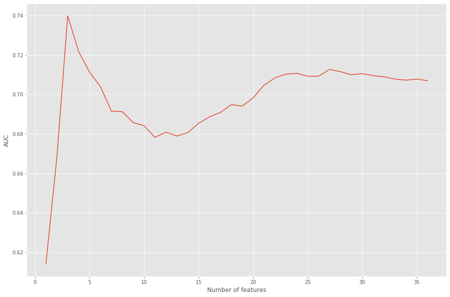
plt.plot(range(1, len(rfecv_rfc.grid_scores_) + 1), rfecv_rfc.grid_scores_)
plt.show()
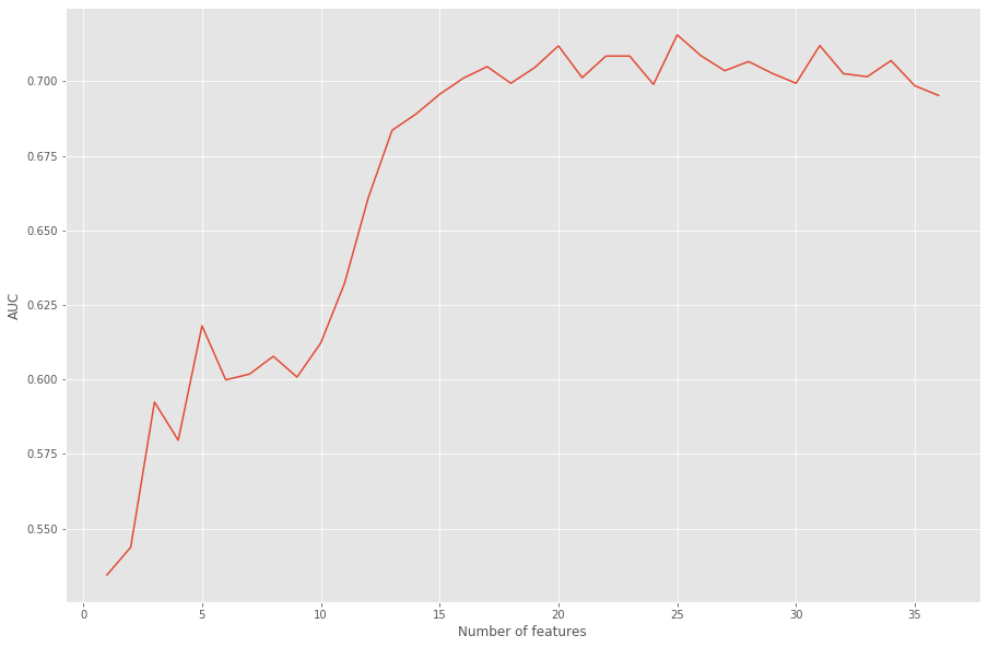
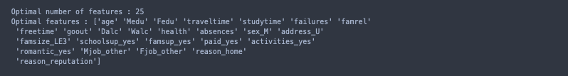
We can see that the best AUC score from our model occurs when only 25 of the 36 transformed features are used as input. This translates to excluding three of the original features entirely: ‘nursery’, ‘internet’, and ‘guardian’.
Hyperparameter Tuning
I’ll now perform a grid search on the model using the selected features.
1
2
3
4
5
6
7
8
9
10
11
12
13
14
15
16
17
18
19
20
from sklearn.model_selection import GridSearchCV

# instantiate parameter grid
rfc_grid = {
            "n_estimators": np.arange(100, 501, 100),
            "criterion": ["gini", "entropy"],
            "max_features": [None, "sqrt", "log2"],
            "max_depth": [None, 5, 10, 15, 20],
            "min_samples_split": [2, 5, 10, 20],
            "min_samples_leaf": [1, 3, 5]
            }

# cross-validated grid search
rfc_gscv = GridSearchCV(rfc, rfc_grid, cv= 5, scoring= 'roc_auc')
rfc_gscv.fit(X_Dummy[best_rfc_feats], Y_train)

# results
print(rfc_gscv.best_score_)
pct_change(old= max(rfecv_rfc.grid_scores_), new= rfc_gscv.best_score_)
print(rfc_gscv.best_params_)

The best set of parameters improved the AUC score by 7.74%.
An AUC of 0.5 is no better than randomly guessing, and a 1.0 would be perfectly seperating the group of passing students from the group who failed. The random forest model is right in the middle with an AUC score of 0.77. As long as the model performs better than random, I’ve done good.. right?
Well, let’s just say that I hope the logistic regression model performs better.
Logistic Regression
Here, I’ll be using the same methods of feature selection and parameter tuning that I used for the random forest model.
Feature Selection
1
2
3
4
5
6
7
8
9
10
11
12
13
14
15
16
17
18
19
20
21
# recursive feature elimination
rfecv_logreg = RFECV(estimator=logreg,
              step=1,
              cv= rep_kfold2,
              scoring='roc_auc')
rfecv_logreg.fit_transform(X_Dummy, Y_train);

# optimal number of features selected for logreg
print("Optimal number of features :", rfecv_logreg.n_features_)

# optimal feature set for logreg
best_logreg_feats = X_Dummy.columns[rfecv_logreg.get_support(indices= True)].values
print("Optimal features :", best_logreg_feats)

# plot number of features VS. AUC scores
plt.style.use('ggplot')
plt.figure(figsize=(15,10))
plt.xlabel("Number of features")
plt.ylabel("AUC")
plt.plot(range(1, len(rfecv_logreg.grid_scores_) + 1), rfecv_logreg.grid_scores_)
plt.show()

Only three of the 36 features were selected, which doesn’t seem right. This is because sklearn’s logistic regression model uses l2 regularization by default.
L2 regularization (ridge regression) applies penalty to the model for added complexity, which is great if the input doesn’t contain any irrelevant features because then it’ll only penalize for repititive features.
L1 regularization (lasso regression) assigns coefficients to the features based on their respective importances. The coefficients of the irrelevant features simply shrink to zero, and are ignored from the model; no penalty is applied.
Using only three features as input doesn’t seem too reliable, so instead, I’ll fit a new model to see which features get excluded by lasso.
1
2
3
4
5
6
7
8
9
10
11
12
13
from sklearn.feature_selection import SelectFromModel

# logreg using l1 regularization
lassoLR = LogisticRegression(penalty= 'l1', max_iter= 2000, solver= 'liblinear')

# feature selector
sel_ = SelectFromModel(lassoLR)
sel_.fit(X_Dummy, Y_train)

# selected features
best_lassoLR_feats = X_Dummy.columns[sel_.get_support(indices= True)].values
print("Number of features :", len(best_lassoLR_feats))
print(best_lassoLR_feats)

This seems more likely.
One of the additional benefits of logistic regression is that if the set still contains any useless features, the model will naturally ignore them.
Hyperparameter Tuning
First, I’ll fit and compare the search results of two different grids. This is primarily to compare lasso vs. ridge regression as the method of regularization. The grids also contain the eligible solvers for each method, and an array of ‘C’ values.
‘solver’ - The solver is just an itterative procedure used for minimizing the convex cost function. A variety approximation methods have been developed over the years, each have their own pro’s and con’s, but their results generally don’t differentiate enough to matter. For small datasets, the selection is somewhat arbitrary.
‘C’ - Finding the best value for ‘C’ is by far more important than choosing a solver. This parameter determines the strength of regularization; the higher the value, the less regularization.
1
2
3
4
5
6
7
8
9
10
11
12
13
14
15
16
17
18
19
20
21
22
23
24
25
26
# instantiate logreg-lasso parameter grid
logreg_l1_grid = { "penalty": ['l1'],
                   "max_iter": [2000],
                   "C": np.linspace(0,100,21),
                   "solver": ['liblinear', 'saga']}

# instantiate logreg-ridge parameter grid
logreg_l2_grid = { "penalty": ['l2'],
                   "max_iter": [2000],
                   "C": np.linspace(0,100,21),
                   "solver": ['liblinear', 'saga', 'sag', 'newton-cg', 'lbfgs']}


# logreg-lasso CV grid search
logreg_l1_gscv = GridSearchCV(logreg, logreg_l1_grid, cv= 5, scoring= 'roc_auc')
logreg_l1_gscv.fit(X_Dummy[best_lassoLR_feats], Y_train)
print('Logistic Regression w/ Lasso - Results')
print(logreg_l1_gscv.best_score_)
print(logreg_l1_gscv.best_params_)

# logreg-ridge CV grid search
logreg_l2_gscv = GridSearchCV(logreg, logreg_l2_grid, cv= 5, scoring= 'roc_auc')
logreg_l2_gscv.fit(X_Dummy[best_lassoLR_feats], Y_train)
print('Logistic Regression w/ Ridge - Results')
print(logreg_l2_gscv.best_score_)
print(logreg_l2_gscv.best_params_)
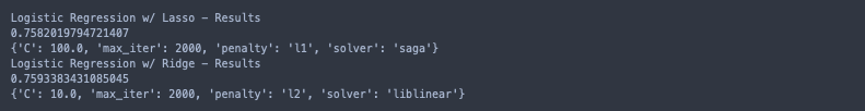
Using l2 regularization results in a slighly better performing model, and the increased values of ‘C’ imply that less regularization was needed. To me, these results are indicative of successful feature selection!
Now I’ll focus on fine-tuning the regularization strength.
1
2
3
4
5
6
7
8
9
10
11
12
# logreg with l2 regularization
logreg2 = LogisticRegression(penalty= 'l2', max_iter= 2000, solver= 'liblinear')

# testing 100 values for C within its known optimal range
C_grid = {"C": np.linspace(7.5, 12.5, 100)}
C_gscv = GridSearchCV(logreg2, C_grid, cv= 5, scoring= 'roc_auc')
C_gscv.fit(X_Dummy[best_lassoLR_feats], Y_train)

print(C_gscv.best_score_)
# AUC inc/dec from C = 10
print(pct_change(logreg_l2_gscv.best_score_, C_gscv.best_score_))
print(C_gscv.best_params_)

No performance increase from the refined search; C = 10 is optimal.
Model Performance
It’s finally time to test the models on unseen data!

First, I need to make new X_train and X_test sets for both models so that they include only their best features (respectively).
1
2
3
4
5
6
7
8
9
10
11
12
13
14
15
16
17
18
19
20
21
22
23
24
25
26
27
28
29
30
31
32
33
34
35
36
37
38
39
40
41
42
43
44
# irrelevant features for Random Forest
RFCfeat_drop = ['nursery', 'internet', 'guardian']

# irrelevant features for Logistic Regression
LRfeat_drop = ['freetime', 'Dalc', 'absences', 'activities', 'nursery', 'guardian']


# multi-categorical feature changes for Random Forest
# unselected category -> 'un_imp'
RFCfeat_replace = {'Mjob' : {'at_home' : 'un_imp',
                             'health' : 'un_imp',
                             'teacher' : 'un_imp',
                             'services' : 'un_imp'
                            },
                   'Fjob' : {'at_home' : 'un_imp',
                             'health' : 'un_imp',
                             'teacher' : 'un_imp',
                             'services' : 'un_imp'
                            },
                   'reason' : {'course' : 'un_imp',
                               'other' : 'un_imp'
                              }}

# multi-categorical feature changes for Logistic Regression
# unselected category -> 'un_imp'
LRfeat_replace = {'Mjob' : {'at_home' : 'un_imp',
                            'health' : 'un_imp'
                           },
                  'Fjob' : {'at_home':'un_imp',
                            'other':'un_imp',
                            'services':'un_imp'
                           }}

# New RFC Train/Test Sets
X_train_rfc = X_train.drop(columns= RFCfeat_drop)
X_test_rfc = X_test.drop(columns= RFCfeat_drop)
X_train_rfc.replace(RFCfeat_replace, inplace = True)
X_test_rfc.replace(RFCfeat_replace, inplace = True)

# New LogReg Train/Test Sets
X_train_lr = X_train.drop(columns= LRfeat_drop)
X_test_lr = X_test.drop(columns= LRfeat_drop)
X_train_lr.replace(LRfeat_replace, inplace= True)
X_test_lr.replace(LRfeat_replace, inplace= True)
The models will also require slightly different preprocessors since they won’t be taking the same input.
1
2
3
4
5
6
7
8
9
10
11
12
13
14
15
16
17
# seperating data types for preprocessing - RFC
num_feats_rfc = X_train_rfc.select_dtypes('int').columns.to_list()
cat_feats_rfc = X_train_rfc.select_dtypes('object').columns.to_list()

# seperating data types for preprocessing - LogReg
num_feats_lr = X_train_lr.select_dtypes('int').columns.to_list()
cat_feats_lr = X_train_lr.select_dtypes('object').columns.to_list()

# Random Forest preprocessor
preprocessor_rfc = make_column_transformer(
                        (MinMaxScaler(), num_feats_rfc),
                        (OneHotEncoder(drop= 'first'), cat_feats_rfc))

# Logistic Regression preprocessor
preprocessor_lr = make_column_transformer(
                        (MinMaxScaler(), num_feats_lr),
                        (OneHotEncoder(drop= 'first'), cat_feats_lr))


I’ll also compute the CV scores for the final models since I haven’t done so already; if I overfit the models, a comparison of accuracies should hint towards how much overfitting is present.
1
2
3
4
5
6
7
8
9
10
11
12
13
14
15
16
17
18
19
20
21
22
23
24
25
# Instantiate Final Models
RFC_model = rfc_gscv.best_estimator_
LogReg_model = logreg_l2_gscv.best_estimator_

# Make Pipelines
RFC_pipe = make_pipeline(preprocessor_rfc, RFC_model)
LogReg_pipe = make_pipeline(preprocessor_lr, LogReg_model)

# Compute CV Scores on Training Data
CVscore_RFC = cross_val_score(RFC_pipe, X_train_rfc, Y_train, cv= 10, scoring= 'accuracy').mean()
CVscore_LogReg = cross_val_score(LogReg_pipe, X_train_lr, Y_train, cv= 10, scoring= 'accuracy').mean()

# Train the Models
RFC_pipe.fit(X_train_rfc, Y_train)
LogReg_pipe.fit(X_train_lr, Y_train)

# Predict on Test Sets
Test_RFC = RFC_pipe.score(X_test_rfc, Y_test)
Test_LogReg = LogReg_pipe.score(X_test_lr, Y_test)

# Results
print("RFC CV Accuracy :", np.round(CVscore_RFC*100, 2), "%")
print("LogReg CV Accuracy :", np.round(CVscore_LogReg*100, 2), "%")
print("RFC Prediction Accuracy :", np.round(Test_RFC*100, 2), "%")
print("LogReg Prediction Accuracy :", np.round(Test_LogReg*100, 2), "%")

Conclusion
Both models were slighly overfit, logistic regression wasn’t bad though. However, neither performed as well as I had hoped. With this being my first project in machine learning, I was very determined to obtain high accuracy. After much more effort afterwards, I realized it can’t be done.
- At first, I continued studying and researching random forest and logistic regression in attempt to improve both models.
- Then, I experimented with different models. Many, many different models.
- Using logistic regression as a ‘meta model’, I made a stacked ensemble of classifiers to generate multiple predictions to predict off of.
- I even used regression models to estimate the individual G1, G2, and G3 test scores to use as additional features in my models here. Still, I had no luck.
Some of the models performed a bit better than these here, but some also performed worse. However, I learned a very valuable lesson here:
If the data won’t tell you what you want to hear, it’s probably because it can’t.
It turns out that the best predictor for whether or not a student will pass or fail a course is their track record. Another user on Kaggle posted their study with G1 and G2 included as features, and they acheived a classification accuracy of 90%.
Of course, it would be very interesting (and just down-right cool) to be able to accurately predict any given students mathematical ability without ever looking at their transcript, but the result is still valuable nonetheless. For instance, devoting a bit more time to explore this concept in depth, educators could potentially make long term success predictions using only the student’s early academic tendencies. Even more importantly, this could assist K-12 schools identify their “at-risk” students early on so they don’t go unnoticed, and to ensure that they get the support and additional attention they need.
Post-Op: Continued Study
2 weeks later …
As I may have hinted at earlier, I wasn’t exactly “satisified” with my results. Given how much time and effort I devoted to this, I wasn’t quite ready to wave goodbye to my first ML project just yet. I decided to refine my predictive capacity, and focus on a more niche group: the honor roll students.
In sum, I essentially just repeated this process, but used 16 as my threshold for ‘G3’ rather than 12. My top performing model was a random forest, which achieved a classification accuracy of 91.6%! It turns out that the honor roll students have a lot in common!
In no specific order, the most important features were:
- age
- health
- weekly alcohol consumption
- parents’ education levels (both)
- quality of family relationships
I may decide to create a seperate post for this later, but I’d like to keep my “My First Machine Learning Project” genuine. So for now, I’ll just leave you with the results. I welcome all forms of criticism and/or advice, and the best way to get in contact with me is through LinkedIn!
If you’ve made it this far, thank you so very much. I hope that you’ve found reading this post as enjoyble as I found making it!
- Drew Woods